Usetex Demo

import matplotlib
matplotlib.rc('text', usetex=True)
import matplotlib.pyplot as plt
import numpy as np

# interface tracking profiles
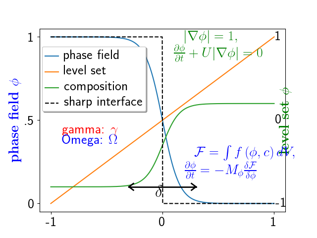
N = 500
delta = 0.6
X = np.linspace(-1, 1, N)
plt.plot(X, (1 - np.tanh(4 * X / delta)) / 2,    # phase field tanh profiles
         X, (X + 1) / 2,                         # level set distance function
         X, (1.4 + np.tanh(4 * X / delta)) / 4,  # composition profile
         X, X < 0, 'k--')                        # sharp interface

# legend
plt.legend(('phase field', 'level set', 'composition', 'sharp interface'),
           shadow=True, loc=(0.01, 0.55))

ltext = plt.gca().get_legend().get_texts()
plt.setp(ltext[0], fontsize=20)
plt.setp(ltext[1], fontsize=20)
plt.setp(ltext[2], fontsize=20)
plt.setp(ltext[3], fontsize=20)

# the arrow
height = 0.1
offset = 0.02
plt.plot((-delta / 2., delta / 2), (height, height), 'k', linewidth=2)
plt.plot((-delta / 2, -delta / 2 + offset * 2), (height, height - offset),
         'k', linewidth=2)
plt.plot((-delta / 2, -delta / 2 + offset * 2), (height, height + offset),
         'k', linewidth=2)
plt.plot((delta / 2, delta / 2 - offset * 2), (height, height - offset),
         'k', linewidth=2)
plt.plot((delta / 2, delta / 2 - offset * 2), (height, height + offset),
         'k', linewidth=2)
plt.text(-0.06, height - 0.06, r'$\delta$', {'color': 'k', 'fontsize': 24})

# X-axis label
plt.xticks((-1, 0, 1), ('-1', '0', '1'), color='k', size=20)

# Left Y-axis labels
plt.ylabel(r'\bf{phase field} $\phi$', {'color': 'b', 'fontsize': 20})
plt.yticks((0, 0.5, 1), ('0', '.5', '1'), color='k', size=20)

# Right Y-axis labels
plt.text(1.05, 0.5, r"\bf{level set} $\phi$", {'color': 'g', 'fontsize': 20},
         horizontalalignment='left',
         verticalalignment='center',
         rotation=90,
         clip_on=False)
plt.text(1.01, -0.02, "-1", {'color': 'k', 'fontsize': 20})
plt.text(1.01, 0.98, "1", {'color': 'k', 'fontsize': 20})
plt.text(1.01, 0.48, "0", {'color': 'k', 'fontsize': 20})

# level set equations
plt.text(0.1, 0.85,
         r'$|\nabla\phi| = 1,$ \newline $ \frac{\partial \phi}{\partial t}'
         r'+ U|\nabla \phi| = 0$',
         {'color': 'g', 'fontsize': 20})

# phase field equations
plt.text(0.2, 0.15,
         r'$\mathcal{F} = \int f\left( \phi, c \right) dV,$ \newline '
         r'$ \frac{ \partial \phi } { \partial t } = -M_{ \phi } '
         r'\frac{ \delta \mathcal{F} } { \delta \phi }$',
         {'color': 'b', 'fontsize': 20})

# these went wrong in pdf in a previous version
plt.text(-.9, .42, r'gamma: $\gamma$', {'color': 'r', 'fontsize': 20})
plt.text(-.9, .36, r'Omega: $\Omega$', {'color': 'b', 'fontsize': 20})

plt.show()

Total running time of the script: ( 0 minutes 0.027 seconds)