
"""
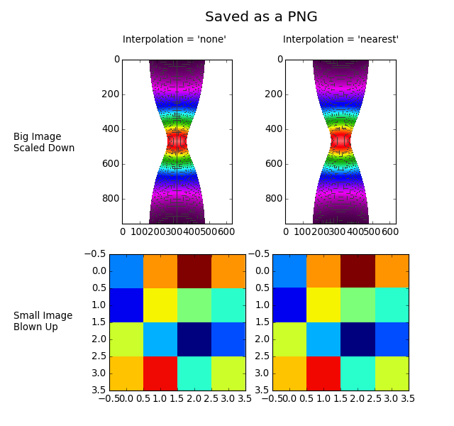
Displays the difference between interpolation = 'none' and
interpolation = 'nearest'.
Interpolation = 'none' and interpolation = 'nearest' are equivalent when
converting a figure to an image file, such as a PNG.
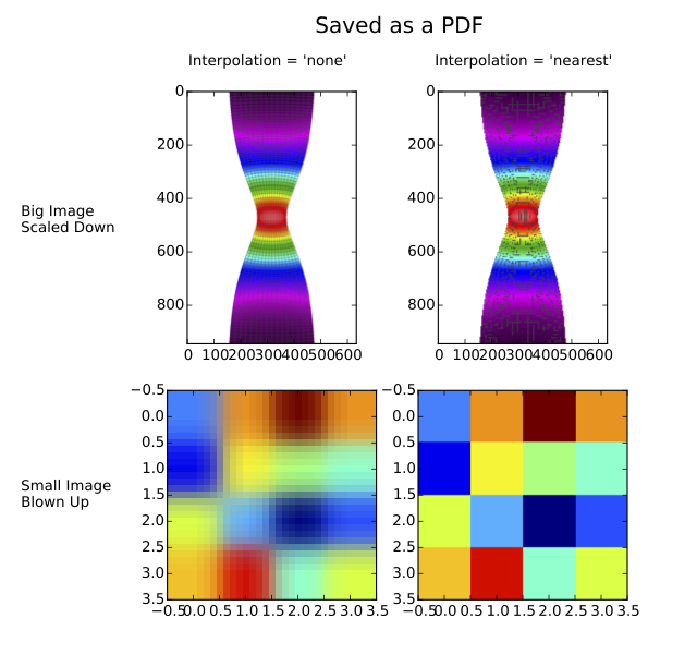
Interpolation = 'none' and interpolation = 'nearest' behave quite
differently, however, when converting a figure to a vector graphics file,
such as a PDF. As shown, Interpolation = 'none' works well when a big
image is scaled down, while interpolation = 'nearest' works well when a
small image is blown up.
"""
import numpy as np
import matplotlib.pyplot as plt
import matplotlib.cbook as cbook
#Load big image
big_im_path = cbook.get_sample_data('necked_tensile_specimen.png')
big_im = plt.imread(big_im_path)
#Define small image
small_im = np.array([[0.25, 0.75, 1.0, 0.75], [0.1, 0.65, 0.5, 0.4], \
[0.6, 0.3, 0.0, 0.2], [0.7, 0.9, 0.4, 0.6]])
#Create a 2x2 table of plots
fig = plt.figure(figsize = [8.0, 7.5])
ax = plt.subplot(2,2,1)
ax.imshow(big_im, interpolation = 'none')
ax = plt.subplot(2,2,2)
ax.imshow(big_im, interpolation = 'nearest')
ax = plt.subplot(2,2,3)
ax.imshow(small_im, interpolation = 'none')
ax = plt.subplot(2,2,4)
ax.imshow(small_im, interpolation = 'nearest')
plt.subplots_adjust(left = 0.24, wspace = 0.2, hspace = 0.1, \
bottom = 0.05, top = 0.86)
#Label the rows and columns of the table
fig.text(0.03, 0.645, 'Big Image\nScaled Down', ha = 'left')
fig.text(0.03, 0.225, 'Small Image\nBlown Up', ha = 'left')
fig.text(0.383, 0.90, "Interpolation = 'none'", ha = 'center')
fig.text(0.75, 0.90, "Interpolation = 'nearest'", ha = 'center')
#If you were going to run this example on your local machine, you
#would save the figure as a PNG, save the same figure as a PDF, and
#then compare them. The following code would suffice.
txt = fig.text(0.452, 0.95, 'Saved as a PNG', fontsize = 18)
# plt.savefig('None_vs_nearest-png.png')
# txt.set_text('Saved as a PDF')
# plt.savefig('None_vs_nearest-pdf.pdf')
#Here, however, we need to display the PDF on a webpage, which means
#the PDF must be converted into an image. For the purposes of this
#example, the 'Nearest_vs_none-pdf.pdf' has been pre-converted into
#'Nearest_vs_none-pdf.png' at 80 dpi. We simply need to load and
#display it.
pdf_im_path = cbook.get_sample_data('None_vs_nearest-pdf.png')
pdf_im = plt.imread(pdf_im_path)
fig2 = plt.figure(figsize = [8.0, 7.5])
plt.figimage(pdf_im)
plt.show()
Keywords: python, matplotlib, pylab, example, codex (see Search examples)

